Microstudies: Part 3
Is 🎶 workin' 9-to-5 🎶 a way to get a degree?
Dolly Parton's hit track "9 to 5" laments the woes of workin' 9 to 5 while barely gettin' by. Despite this treatise against work and the plight of the white-collar worker, many people still believe that in the case of youths, a job will "do them some good".
In a way, I agree — I worked in a café during my teenage years and feel my experience working in hospitality has made me vaguely more well-rounded. At least, I noticed this when I moved to student halls for my university study and had to interact with people who had, in their 18 years, never had to work a day in their life. However, working might be less of a fun personality-building exercise when it becomes less of a fun side-job and instead becomes a necessity — particularly if work might get in the way of study.
In this microstudy, I explore the relationship between student workloads and course grades.
Specifically, the hypotheses being tested are:
: Students who report being in paid employment will attain lower test scores than students who report not being employed.
: Students who are enrolled in more courses attain lower test scores than students enrolled in fewer courses.
: There will be a negative correlation between students' estimated total workload and test scores.
More or less — the hypothesis is that students who have a higher workload will get lower test scores.
Method
The data collected for this study was gathered from a CS1 course designed for students who have no prior programming experience that teaches the basics of imperative programming using the Python programming language. The course has four computer-based tests spread throughout the semester run asynchronously during students' normal lab times. Data were collected over two semesters in 2024 — with the first semester acting as a pilot for the second. The questionnaire data in this study were gathered in Test 3 for both semesters.
The Pilot
The pilot study was conducted during the summer semester (Jan – Feb) which is an intense 6-week semester (compared to the usual 15-week semester at the institution). In total, there were 84 students enrolled in the course.
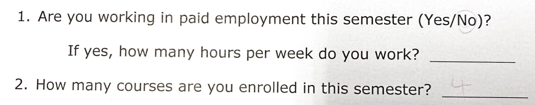
Students fill in a paper attendance sheet at the start of each test that they must hand in before leaving the room. Beneath the name, ID, and seat number fields, I asked the teaching team to add the following questions:
The Main Study
The main study was conducted during semester 1 (March – June) which is run over 15 weeks. In total, there were 676 students enrolled in the course.
The question given to students was not modified between the pilot and main study.
Results
As in microstudy part 2, I am interested in the effect of employment and workload on test scores across all four tests. To analyse this, I took the average grades across all four tests for each student — ignoring missing test grades.
The Pilot
For the pilot study run during the summer semester, 75 out of the 84 enrolled students sat the test, and of those, 67 students (89%) responded to the questionnaire. Only the data of those students who responded to the questionnaire will be used further.
The mean and median test scores were 66.5% and 65.6% respectively.
Employment
Of the 67 students who responded to the questionnaire, 33 (49%) reported being in paid employment, and 34 (51%) reported not being in paid employment. The distribution of test scores is below:
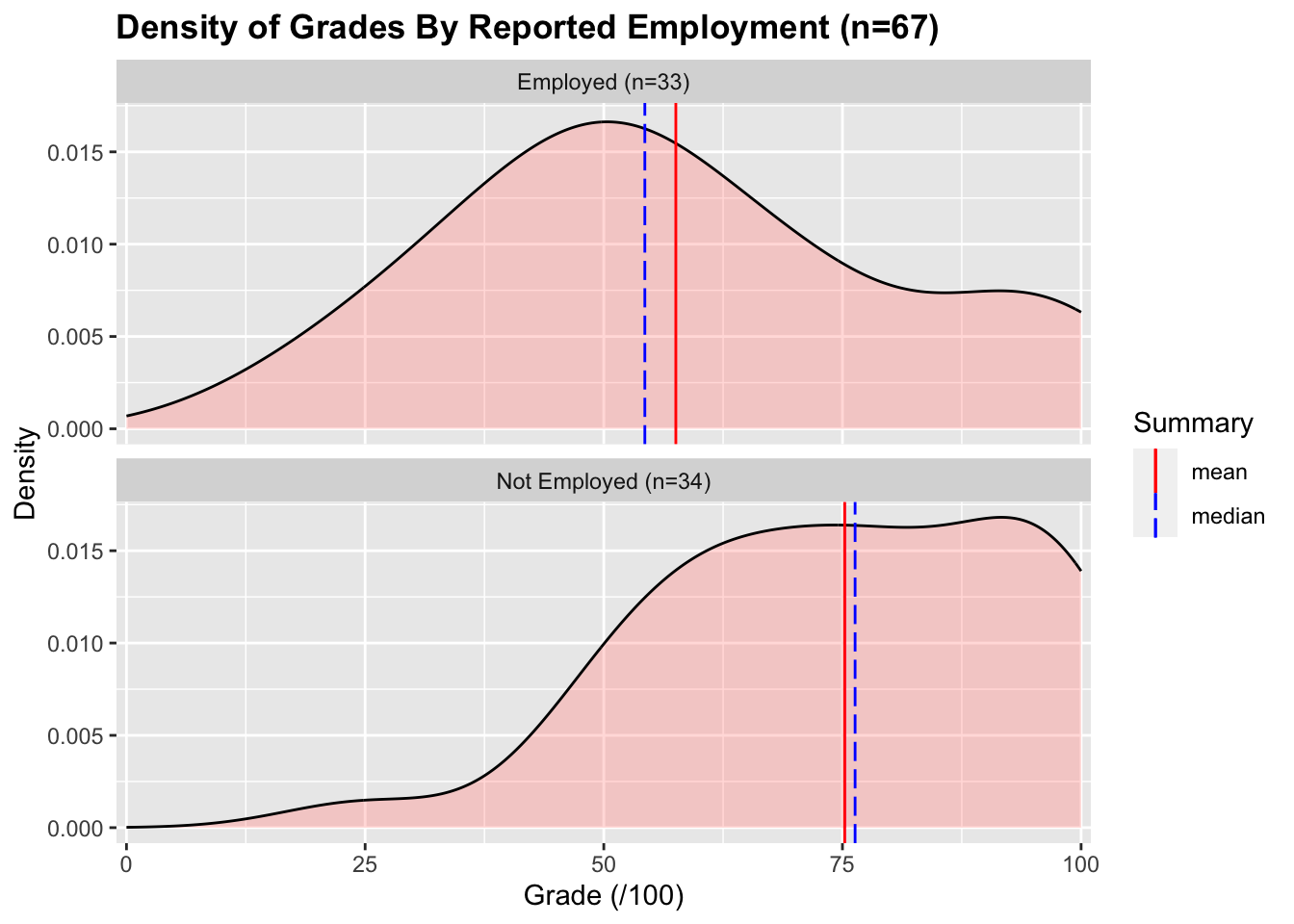
The mean and median test scores for the employed group is 57.5% and 54.3% respectively. The mean and median for the not employed group is 75.2% and 76.3% respectively. The difference between these two groups is significant1 with a medium effect size2.
Hours Worked
The students who reported being in paid employment reported a mean and median weekly workload of 18.8 hours and 15 hours respectively. The distribution of the hours worked per week is below:
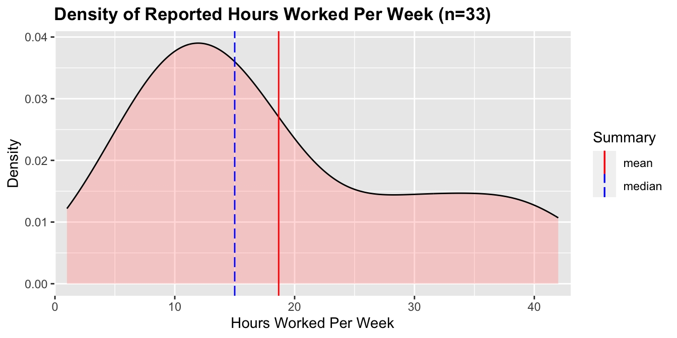
Note: for students who put ranges of hours (e.g. "5–7"), the average of the range was recorded.
There is no correlation between the hours worked per week and grades3
Coursework
During summer school, it is common for students to only take one course. Students can enroll in a maximum of two courses during the summer semester. Of the 67 students who responded to the questionnaire, 39 (58%) were enrolled in one course and 28 (42%) were enrolled in two courses. The grade distributions are below:
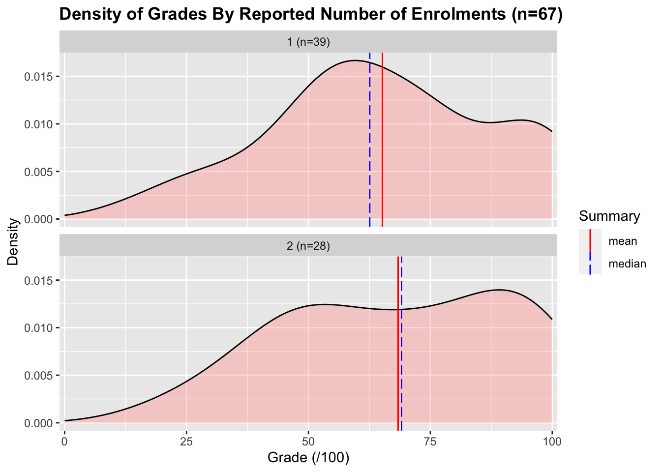
The mean and median test scores for students taking one course were 65.1% and 62.6% respectively. The mean and median test scores for students taking two courses was 68.4% and 69.1% respectively. There is no significant decrease in grades between the one- and two-course groups4. In fact, the grades for the two-course group appear slightly higher than for the one-course group.
Estimated Workload
The breakdown of employment and course enrolments is below:
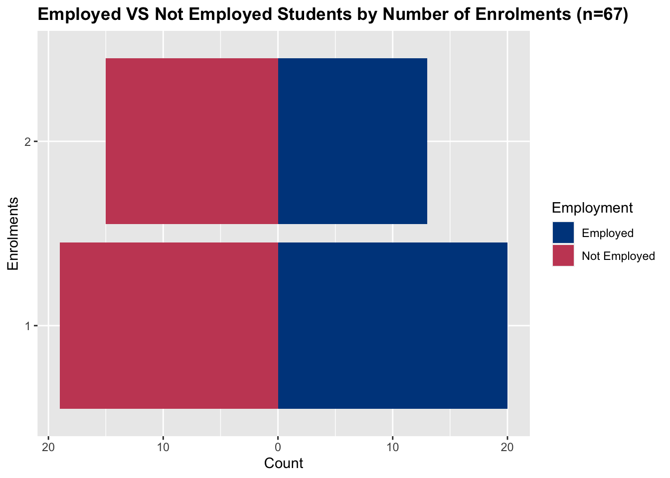
I have looked at the employment and enrolments of students individually; however, to combine these values, I estimate the weekly number of hours of work for each student. During summer school, students are expected to spend 20 hours studying for each course (this includes the time they spend in lectures and labs). An overall estimate is then calculated for each student by summing this expected coursework workload with the reported hours worked per week (if the student reports working). The distribution of estimated workload is below:
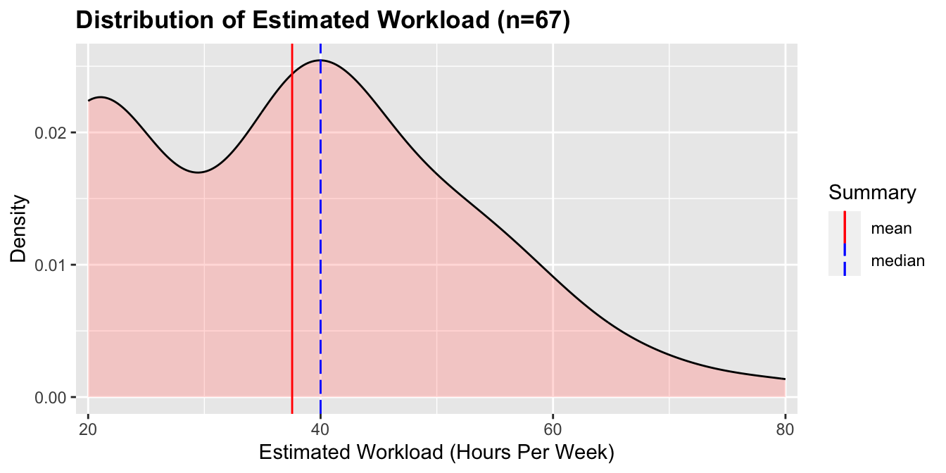
Students had a mean and median estimated workload of 37.6 and 40 hours per week respectively, with most students having an estimated workload of 40 hours.
The estimated workload is plotted against test scores below:
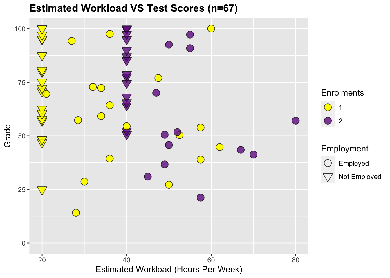
There is a very weak negative correlation between the estimated workload per week and test scores5.
The Main Study
For the main study run during semester 1, 591 of the 676 enrolled students sat the test, and of those 552 students (93%) responded to the questionnaire.
The mean and median test scores were 63.8% and 67.5% respectively.
Employment
Of the 552 students who responded to the questionnaire, 205 (37%) reported being in paid employment, and 347 (63%) reported not being in paid employment. The distribution of test scores for the two groups is below:
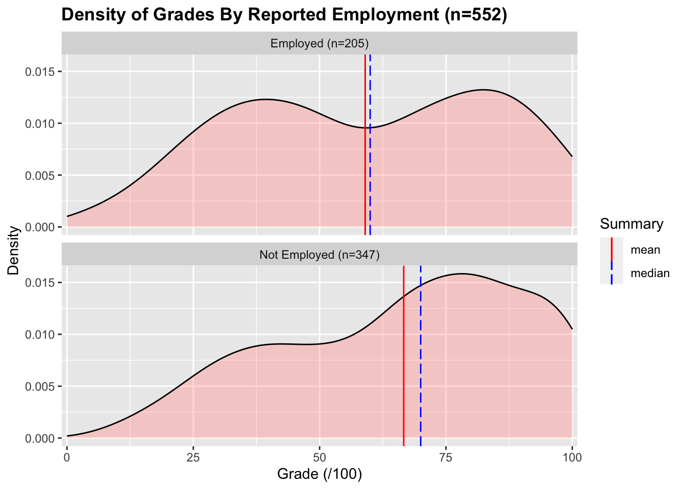
The mean and median test scores for the employed group are 59.0% and 60.0% respectively. The mean and median test scores for the not employed group are 66.6% and 70.0% respectively. The grades for the employed group are significantly lower than the grades for the not employed group6 with a small effect size7.
Hours Worked
The students who reported being in paid employment reported a mean and median weekly workload of 12.9 hours and 11 hours respectively. The distribution of the hours worked per week is below:
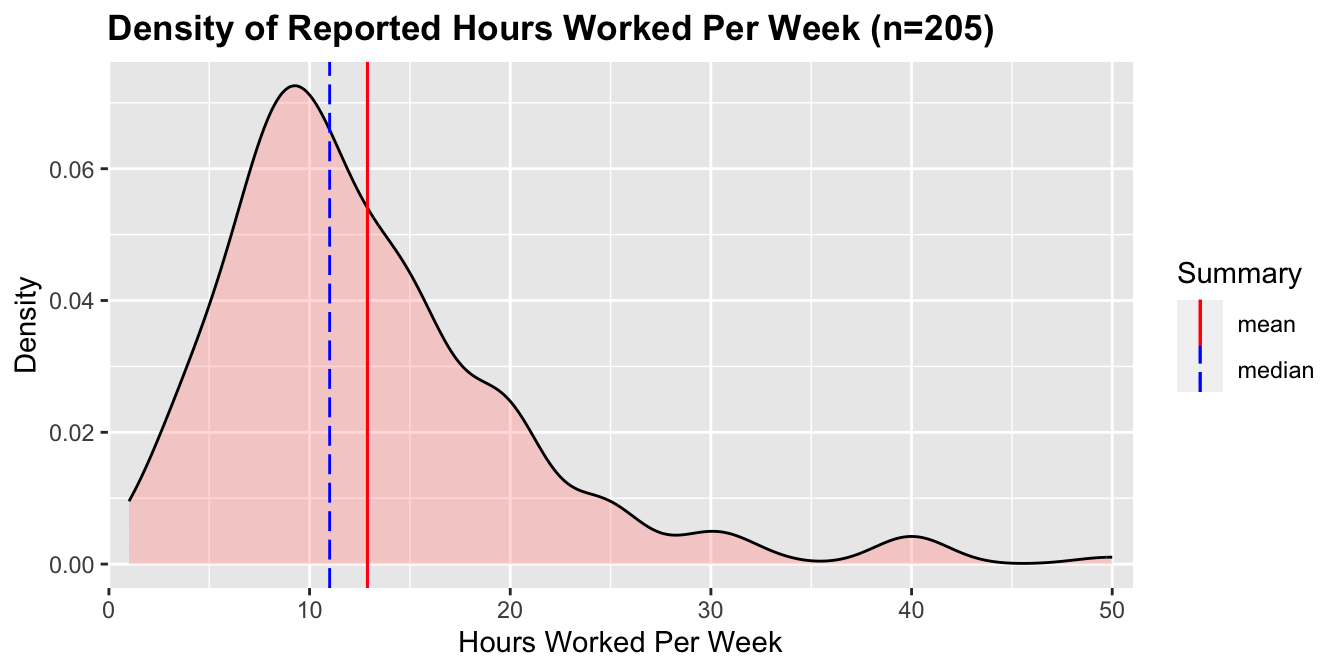
There is no correlation between the hours worked and grades8
Coursework
During regular semesters, it is common for students to take four courses. Students can enrol in a maximum of five courses. The breakdown of enrolments and average test scores is below:
| #Courses | n | n% | Mean (%) | Median (%) |
|---|---|---|---|---|
| 1 | 8 | 1.5 | 77.68 | 80.93 |
| 2 | 7 | 1.3 | 64.28 | 70.00 |
| 3 | 33 | 6.0 | 62.77 | 67.50 |
| 4 | 462 | 83.7 | 63.23 | 66.97 |
| 5 | 42 | 7.6 | 68.17 | 78.41 |
The grade distributions of these groups are below:
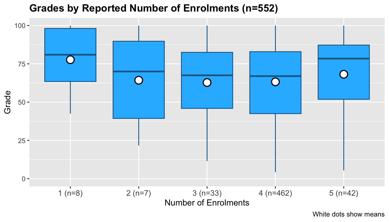
A Spearman's rank correlation test shows no correlation between the number of enrolments and grades9.
Estimated Workload
The breakdown of enrolments and employment is below:
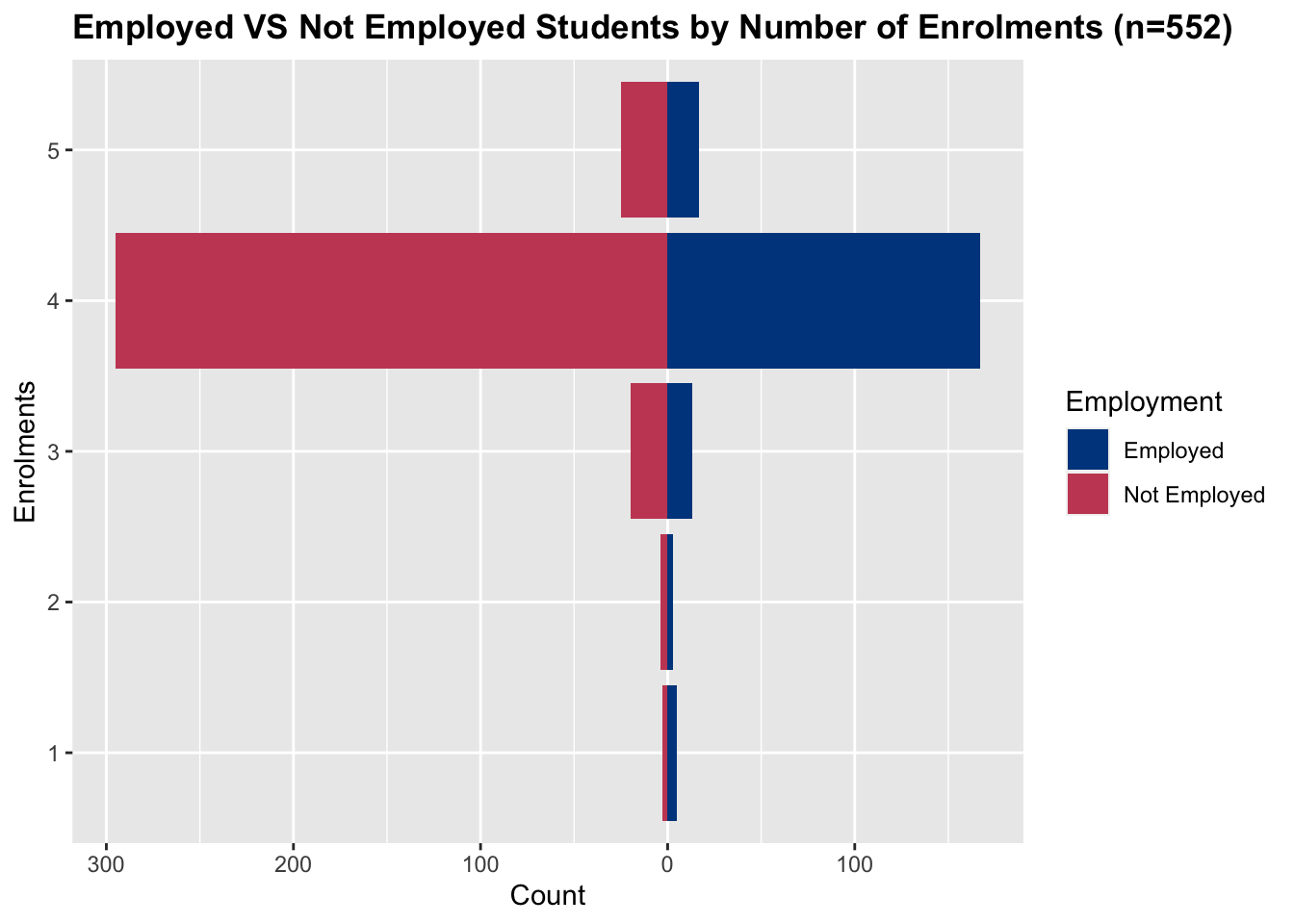
As in the pilot, an estimate of student workload in hours per week is calculated. During normal semesters, students are expected to spend 10 hours studying for each course (this includes the time they spend in lectures and labs). An overall estimate is then calculated for each student by summing this expected coursework workload with the reported hours worked per week (if the student reports working). The distribution of estimated workload is below:
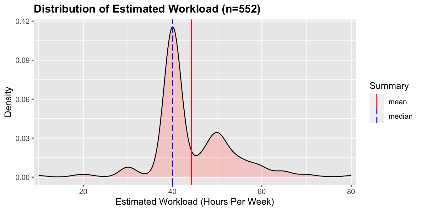
Students had a mean and median estimated workload of 44.3 and 40 hours per week respectively, with most students having an estimated workload of 40 hours.
The estimated workload is plotted against test scores below:
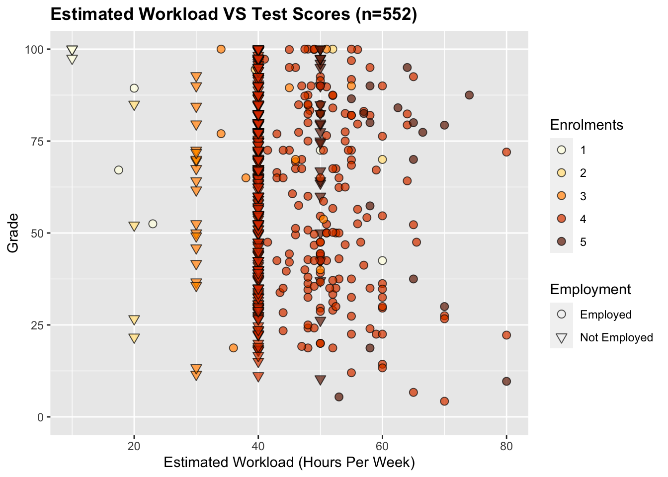
There is a very weak negative correlation between the estimated workload per week and test scores10.
Discussion
Who knew you could fit so many density plots on to one little blog post! So far, the messiest microstudy.
There seems to be no correlation between the number of hours worked per week and grades, number of enrolled courses and grades, and not even the combination of the two — the estimated workload and grades. Despite this, there is a consistent drop in grades between the not employed students and the employed students across both semesters — but this effect is small.
From this we can tentatively accept and outright reject and — there doesn't seem to be any significant correlation between the number of course enrolments and grades, nor the overall estimated workload and grades; however, being employed seems to slightly negatively impact grades regardless of the number of hours worked or course enrolments.
Limitations
As with the other microstudies, an obvious limitation of this study is the fact that only two cohorts of students were asked three questions on a self-selected questionnaire at a single institution in New Zealand. These results may not generalize to other countries or institutions.
Conclusions
There are many follow-up questions I wish I could ask: What is the age distribution of the students who are working? What is the nature of their work — office based, or manual labour? Is their place of work close to their homes or the university? Do they mostly work on the weekends, or during the week? If students are working, is it out of necessity or for a bit of extra walking around money? If they could enroll in fewer courses, would they? If they could stop work, would they?
Those last three questions are interesting in the context of a New Zealand university. In addition to a course fees loan, the New Zealand student loan scheme allows students to get an allowance or loan for living costs of up to $316 per week11. However, there is only one first-year student accommodation plan at this university that costs less than this per week — and it is for a twin-share room plan, which is not common in New Zealand. Some eligible students are able to get an additional $60pw as accommodation support12 — but this increased amount of $376 only covers one more first year accommodation plan — with the other accommodation plans costing between $490 and $510 per week11. Amazingly, the apartment that has these two cheapest accommodation plans only has a capacity for 38 students13 — meaning many students living in other student accommodation will be at least $100–130 out per week. Thankfully, these accommodation plans are catered meaning there are no additional food costs.
Doing some back-of-the-napkin math, to cover the additional $100–130 rent and maybe have a scant $50 left over per week for other expenses, students would need to work between 7 and 9 hours per week assuming a minimum wage14 at the lowest tax-bracket15. To reiterate, this is the bare minimum a student who receives living costs in addition to accommodation support would need to work to afford shelter and food in university accommodation.
One suggestion might be for students to enroll in fewer courses and pick up more part-time work on the side to cover this discrepancy. Unfortunately, while working does not affect living cost loan eligibility, studying part-time does16. To be considered full time, students must enrol in seven courses per year (one fewer than the usual eight courses full-time students enrol in)17. This could put some students in a bind — they need to work to afford living costs and so have less time and energy for study, but need to study full time to be eligible for a student loan.
Not to belabour the point — but there is an equity argument to be made here. This study has shown employment has a small but negative impact on test score performance. Many students in the main study are enrolled in four courses (full time) while being in paid employment — obviously, we do not know the circumstances behind this (i.e. whether this is out of necessity or just for extra money) but New Zealand already has a problem with high school students needing to work during study and it would be unsurprising if these issues were to continue at the tertiary level.
Footnotes
-
The grades for the employed/not employed groups are just above the p=0.05 threshold for normality: Employed (W=0.96, p=0.248), Not Employed (W=0.95, p=0.090). However, as, visually, the groups do not appear normal, a more conservative 1-tailed Mann-Whitney test was performed over a t-test yielding: (U=304, p<0.001) ↩
-
A Cliff's delta effect size test gave a statistic of -0.458 with a 95% confidence interval of -0.668 to -0.180 ↩
-
A Spearman's rank correlation gives: r(31) = -0.051, p = 0.777 ↩
-
As before, there is not enough evidence to reject the normality hypothesis: One course (W=0.96, p=0.221), two courses (W=0.94, p=0.138). However, as, visually, the data appears to be non-normal, a more conservative 1-tailed Mann-Whitney test was performed over a t-test yielding: (W=577.5, p=0.658). A cliffs delta shows a negligible effect size: -0.058 with a 95% confidence interval of -0.333–0.226. ↩
-
A Spearman's rank correlation gives: r(65) = -0.241, p = 0.050 ↩
-
The grades for the employed/not employed groups are not normal: Employed (W=0.96, p<1e-5), Not Employed (W=0.95, p<1e-8). A 1-tailed Mann-Whitney test was performed: (U=29695, p<0.001) ↩
-
A Cliff's delta effect size test gave a statistic of -0.165 with a 95% confidence interval of -0.262 to -0.064 ↩
-
A Spearman's rank correlation gives: r(203) = -0.078, p = 0.264 ↩
-
A Spearman's rank correlation gives: r(550) = -0.021, p = 0.622 ↩
-
A Spearman's rank correlation gives: r(550) = -0.118, p = 0.006 ↩
-
Retrieved July 2024: https://www.studylink.govt.nz/products/a-z-products/student-loan/living-costs.html ↩ ↩2
-
Retrieved July 2024: https://www.studylink.govt.nz/products/rates/accommodation-benefit-rates.html ↩
-
Retrieved July 2024: https://www.auckland.ac.nz/en/on-campus/accommodation/accommodation-options/self-catered-accommodation/grafton-student-flats.html ↩
-
Retrieved July 2024: https://www.employment.govt.nz/pay-and-hours/pay-and-wages/minimum-wage/minimum-wage-rates-and-types ↩
-
Retrieved July 2024: https://www.ird.govt.nz/income-tax/income-tax-for-individuals/tax-codes-and-tax-rates-for-individuals/tax-rates-for-individuals ↩
-
Retrieved July 2024: https://www.studylink.govt.nz/starting-study/whats-available/studying-part-time.html ↩
-
Retrieved July 2024: https://www.studylink.govt.nz/about-studylink/glossary/efts.html ↩